Journal:A new numerical method for processing longitudinal data: Clinical applications
| Full article title | A new numerical method for processing longitudinal data: Clinical applications |
|---|---|
| Journal | Epidemiology Biostatistics and Public Health |
| Author(s) | Stura, Ilaria; Perracchione, Emma; Migliaretti, Giuseppe; Cavallo, Franco |
| Author affiliation(s) | Università di Torino, Università di Padova |
| Primary contact | Email: Ilaria dot stura at unito dot it |
| Year published | 2018 |
| Volume and issue | 15(2) |
| Page(s) | e12881 |
| DOI | 10.2427/12881 |
| ISSN | 2282-0930 |
| Distribution license | Creative Commons Attribution-NonCommercial-NoDerivatives 4.0 International |
| Website | https://ebph.it/index.php/ebph/article/view/12881 |
| Download | https://ebph.it/article/view/12881/11630 (PDF) |
|
|
This article contains rendered mathematical formulae. You may require the TeX All the Things plugin for Chrome or the Native MathML add-on and fonts for Firefox if they don't render properly for you. |
Abstract
Background: Processing longitudinal data is a computational issue that arises in many applications, such as in aircraft design, medicine, optimal control, and weather forecasting. Given some longitudinal data, i.e., scattered measurements, the aim consists in approximating the parameters involved in the dynamics of the considered process. For this problem, a large variety of well-known methods have already been developed.
Results: Here, we propose an alternative approach to be used as an effective and accurate tool for the parameters fitting and prediction of individual trajectories from sparse longitudinal data. In particular, our mixed model, that uses radial basis functions (RBFs) combined with stochastic optimization algorithms (SOMs), is here presented and tested on clinical data. Further, we also carry out comparisons with other methods that are widely used in this framework.
Conclusion: The main advantages of the proposed method are the flexibility with respect to the datasets, meaning that it is effective also for truly irregularly distributed data, and its ability to extract reliable information on the evolution of the dynamics.
Keywords: statistical method, radial basis function; stochastic optimization algorithm, longitudinal data
Introduction
Longitudinal data are often the object of study in many fields, e.g., sociology, meteorology, and medicine. In medicine, repeated measurements are used to monitor patients’ behaviors and also to adjust therapies accordingly. However, many problems occur when these data are analyzed. Indeed, each time series could have a different number of observations and not be equally spaced. In addition, the sampling period could vary from patient to patient, and measurement errors and also missing data often occur. Thus, since in these cases common methods such as linear regression usually fail, the recent research is directed towards more robust statistical methods. For instance, longitudinal data are commonly analyzed using parametric models such as Bayesian ones[1], as well as functional data analysis (FDA).[2][3] In both cases, many data are required in order to model the behavior of the studied variable(s). These methods, in fact, try to find an "average curve" using all the data, including truncated series and observations with missing information.
However, in clinical applications the estimate on the future dynamics of a single series, given few previous values, could be needed; think for instance to tumor volumes during a treatment, height/weight of children during growth, and concentration of some substance in the body. Each patient is different and could have different growth behavior and different growth parameters, so an "average curve" could not be sufficient. An important piece of information could be, for example, the possible future development of the subject, given his/her previous growth and the clinical background (e.g., treatments). These data could be compared with the real dynamics, in order to see if the response of the patients to the treatment is stable (the parameters do not vary in the future) or not (change in the parameters).
The aim of our work is to propose our numerical tool that can provide information on the future dynamics given few follow-up data. Thus, we first model longitudinal data via widely used mathematical models in population dynamics. As such, on one hand we aim at validating such a model by approximating the parameters involved in the dynamics. On the other one, we are also interested in giving reliable information on the future dynamics of the curves.
In order to achieve our goal, we propose our numerical tool based on optimization methods coupled with interpolation techniques. Specifically, we approximate the parameters involved in the dynamics by means of stochastic optimization algorithms (SOMs).[4][5][6][7] Moreover, for each data series, we improve the performances of the optimization tools by means of radial basis function (RBF) interpolation; see Fasshauer and McCourt[8] for a general overview and Cavoretto et al.[9][10] for particular instances on the topic and applications. In the interpolation process, we also take into account the critical computational issue of carrying out stable computations. For this reason, and since data are subject to noise, we adopt a kind of Tikhonov regularization.[11]
The method, namely RBF-SOM, is here tested on two different datasets:
- height measurements of children with a diagnosis of growth hormone deficiency (GHD) during treatment, and
- prostate-specific antigen (PSA) values of prostatectomized patients with a recurrence of prostate cancer.
In the next section of this paper, the RBF-SOM technique is described. Afterwards, the two datasets used for the validation are presented. The "Results" section is devoted to the numerical results and it is divided into two subsections: in the first one, all the data of each series are considered in order to reconstruct the curves and approximate the parameters, while, in the second one, only a few initial data of each series are used to predict the curve behavior. The last two sections offer a discussion and conclusions.
Methods
This section is devoted to describe the method used to fit a given data series and to approximate the parameters involved in the dynamics.
Given several scattered measurements sampled at different times , the basic idea of the RBF-SOM here proposed consists in considering the theoretical function f, depending on the time t and on several parameters λ = (λ1,..., λp), and to approximate such parameters in order to obtain reliable information on the biological or physical phenomenon.
In the proposed examples, we use, as theoretical growth curve f, the so-called Gompertzian function:
- ,
where f0 is the measurement at time t0 (i.e., the first measurement), λ1 is the growth rate, and λ2 is the carrying capacity, i.e., the maximum value that can be asymptotically achieved by f.
The Gompertzian function is characterized by a fast-growing initial period and by a progressive slowdown, reaching a carrying capacity after a certain time. This curve, depending on the values of the parameters, is able to model a variety of types of growth, from human to cancer cells.[12][13][14][15][16] For this reason, we will use in Section 5 the same function for both datasets. Moreover, its form is particularly suitable in this study because the parameter estimation is not possible via simple methods like Least Square Approximation.
Trivially, the parameters are approximated by finding
- .
Note that we need optimization methods that can be used in case of non-linearity of f, as in the considered cases. In particular, we direct our research throughout stochastic methods. They have been designed by considering analogies with natural phenomena. The most popular are evolution strategy and genetic algorithms, both based on competition among individuals. On the opposite, other methods proposed in the last decades mainly focus on cooperation. Among them, particle swarm optimization (PSO), cuckoo search (CS), and ant colony are widely used techniques, based on the mutual interaction and exchange of information between individuals. In particular, here we will consider PSO and CS, briefly described in what follows.
PSO has been firstly introduced by Kennedy (social psychologist) and Eberhart (electrical engineer)[4] and was further developed by other researches.[6][7][17] In order to describe it, let us consider a group of particles or birds which are represented as points in the space. At first, we need to model their way of flying. Then, taking into account that the target of birds consists in looking for the maximum availability of food, i.e., the minimum of the objective function f, we can easily find its minimum.
The main objective consists in simulating the trajectories of the single birds by considering their selfish behavior (which is the ability of a bird of randomly flying away from the flock) and their social behavior (which is the ability of a bird of staying in the group). With these simple considerations, it is possible to simulate the way of moving of a group of birds, taking also into account that particles avoid collisions.
To explain how we can find the minimum of the objective function interpreting the latter as food, let us first suppose that a bird discovers some food. Then, the other birds have two alternatives: get out of the flock and reach the food (selfish behavior) or stay in the flock (social behavior).
If a good trade-off between the two behaviors is allowed, then the flock can reach the minimum. Indeed, if a bird can move towards some food, then other birds can change their directions towards the same place. Acting in this way, the flock gradually changes its direction until the best place, i.e., the minimum, is reached.
As concerns CS, it was developed by Yang[18] and it simulates the behavior of the cuckoo, a bird that does not incubate its eggs but tries to put them in nests of other species. The problem of this conduct is that, in some cases, the egg is removed by the nest’s owner. The cuckoo, then, searches for a nest in which its egg can be "confused" with the others. Therefore, in this algorithm the minimum of the function is the nest in which more cuckoos can put their eggs without being discovered.
As for the PSO, the user needs to give a set of possible initial solutions. They are usually randomly initialized. Indeed, if the initial solutions are chosen so that they are feasible, the stochastic methods do not fail into local minima, and thus the methods are not truly sensitive with respect to the initial conditions. The main difference with respect to the PSO approach is that, at each iteration, a fraction of nests, which are far from the minimum, are abandoned and new ones close to the minimum are built.
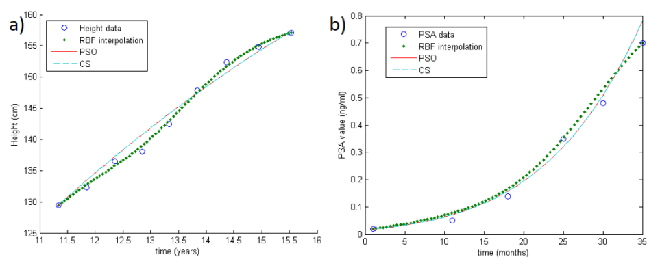
Note that both PSO and CS approaches can be performed in order to minimize the target function, but unfortunately the cardinality of the samples in concrete applications is really small. Thus, in order to improve the performance of the optimization methods, we first reconstruct the growth curves by means of an RBF-based interpolation scheme.[8][9][19] In doing so, we also take into account the instability problems arising in applications. An example of RBF reconstruction can be seen in Fig.1a-b (big colored dots).
|
Moreover, the so-reconstructed function can be used to estimate λl, l > N, i.e., the evolution of the considered quantity.
As an accuracy indicator, we use the following root mean square error:
,
where denotes the number of patients. This indicator represents the standard deviation of the differences between predicted and observed values.
Data
In order to assess strength and weaknesses of the discussed methods, we use two different datasets presented below. Both datasets are real patients’ data. Each patient has a different number of irregularly spaced measurements in a different time interval.
Children data
Different problems can occur during growth. Here we consider pediatric patients with a diagnosis of idiopathic growth hormone deficiency (IGHD), i.e., a low or absent production of GH for unknown causes. These children are treated with rhGH (a synthetic GH) and monitored during growth.
Our dataset is composed by 121 male IGHD patients, treated in “Ospedale Infantile Regina Margherita (OIRM)” in Turin between January 2000 and January 2016.[16][20] Few studies analyze the effect of GH therapy on height, preferring a more indirect approach, where factors influencing the total pubertal and pre-pubertal growth in GH-deficient patients are evaluated and subsequently used to estimate the overall effect at the end of the therapy. Unfortunately, this approach does not quantify the real growth gain in treated patients. Using a non-parametric empirical Bayes approach, our study analyzes the growth response to GH treatment in a homogeneous cohort of 317 patients with pituitary GH deficiency who were enrolled during their pre-pubertal stage in the GH Piedmont Registry (Italy). The measurements are collected every four to six months from the beginning of the therapy (age between 3 and 14 years) to adulthood (18-20 years old). As explained by Gliozzi et al.[12], each period of human growth can be modeled with a Gompertzian law. We therefore use, as a theoretical function, the Gompertz curve explained in the section before.
Note that each series is monotonic, strictly growing, not (or slightly) affected by measurement errors and it has very few missing data. Therefore, we expect robust performances of the RBF-SOM method for this clinical test.
Prostate cancer data
Data released from clinicians about the PSA value (which is a mirror of the mass of the prostate cancer) are needed in order to have a reliable estimate of the cancer’s evolution. After a radical prostatectomy, the PSA turns out to be a good biomarker and could be used to monitor a possible relapse. In fact, only prostate cells produce PSA, and, after surgery, there should be no prostate cells in the body. Hence, the PSA value should be very small, close to zero. If its value is bigger than 0.2 ng/mL, then PSA-producer cells are present, i.e., a relapse (a local or distal metastasis) has occurred.
Here we use a subset of the Eureka1 study collection.[21] Eureka1 is a retrospective study on Italian patients who had a prostatectomy in the last 15 years. Our subset contains follow-up data (PSA values series) of relapsed patients who did not undergo an adjuvant therapy.
In general, cancer growth is very fast and is modeled with an exponential function. However, prostate cancer is a very slow-growing tumor, so Gompertzian[22][23][24] and West[25][26][27] laws are often used. In the following section, we will use the Gompertzian one.
Note that these series are not monotonic: PSA values can grow, be stable for months, or decrease. PSA values should be sampled each four to six months, while in some series only one or two values are reported in one to two years. The PSA value strictly depends on the accuracy of instruments used in the laboratory: some machines have a precision of 0.1 ng/ mL, while others of 0.01 ng/mL. Moreover, the precision could change from value to value in the same series. Therefore, for the RBF-SOM method, this dataset is more challenging than the previous one.
Results
Curve reconstruction
The tests carried out in this subsection are devoted to assess the robustness of the RBF-SOM method as a descriptive tool. Indeed, we consider each growth curve and we approximate the two parameters involved in the dynamics, i.e., the growth rate and carrying capacity. We remark that, at first, we reconstruct the curve by means of RBF interpolants and we then apply PSO or CS methods. The aim of these experiments is to obtain feedback about the accuracy of the proposed approach in approximating the parameters.
Figure 1 (previous) shows two examples of the methods in the case of one unknown parameter. In particular, Fig.1a shows the reconstruction of a growth curve of one child (GH Database), while Fig.1b shows the reconstruction of a PSA growth curve. The circles represent real data, the big colored dots are the RBF interpolation, and the straight and dotted lines are the PSO and CS reconstructions respectively.
For both datasets, we consider as theoretical growth curve the Gompertzian function. Note that, differently from the growth rate, the carrying capacity (the maximum value that can be achieved asymptotically) is supposed to be fixed and known for all patients in both datasets, i.e., only one parameter should be estimated. In what follows, we test the methods with both one and two unknown parameters. As expected, when only the growth rate needs to be estimated, we obtain better results.
More precisely, as concerns only one unknown parameter λ1 (while λ2 is fixed as 200 cm in GH and 200 ng/mL in PSA database) both RBF-PSO and RBF-CS are truly performing and show the same accuracy ( =1.2 cm in GH and =0.9 ng/mL in PSA database). Results are shown in Table 1. This means that data follow the theoretical distribution predicted by the Gompertzian and that the parameter is accurately estimated.
As concerns two unknown parameters, RBF-CS is more effective than RBF-PSO. In fact, for the former the =0.80 cm and =0.89 ng/mL in GH and PSA database, respectively, while for the latter the =2.66 cm and =0.91 ng/mL. Results are shown in Table 1. Note that this happens also enlarging the basin of possible solutions in the CS algorithm.
| ||||||||||||||||||||||||||||||||||||
Dynamics evolution
This subsection is addressed to test the method for modelling the evolution of the dynamics. Thus, we apply the RBF-SOM using only the first four values of each series. We select the first four values for several reasons. First of all, we do it because of data availability: indeed, only a few patients (in both databases) have more than six values in their series. Then, selecting four data points in the databases means that they represent about two years of follow-up, which is a reasonable period to understand the future dynamics.
Again, by fixing the carrying capacity, both methods give the same results ( =3.01 cm in GH and =3.20 ng/mL in PSA database). Results are shown in Table 1 (previous). Of course, the error is larger than the one shown in the previous subsection. However, since here we only take four values, such error indicates a meaningful accuracy on the estimation, especially as concerns the GH case. In fact, it means that, after four measurements, we are able to estimate the final height with a precision of about 3 cm. Looking at the other dataset, the error seems truly large, with =3.20 ng/mL. But, the majority (73.46%) of estimates differ less than 1 ng/mL to the real value. Unfortunately, the irregularity of the measurements and the errors due to the machine precision might cause problems for several series. Indeed, in a few cases (6.12%), results differ more than 3 ng/mL from the real value.
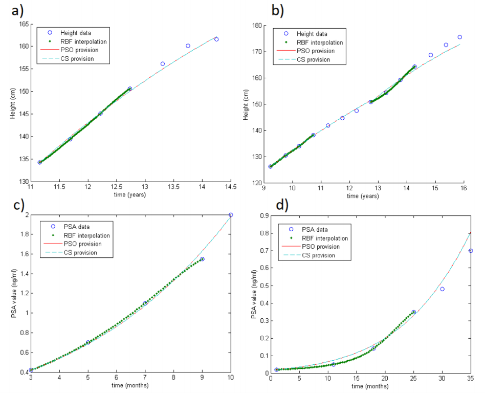
Figure 2 shows some examples of the output of the method, in case of one unknown parameter: the circles are the real data (heights or PSA during visits), dots are the RBF interpolation on the first four values, and PSO and CS provisions are the straight and dotted lines. Fig.2a-b concern the GH database, while Fig.2c-d the PSA database. In particular, Fig.2a shows only one growth period, while in Fig.2b there is the combination of two growth periods. Note in Fig.2d that the estimation error grows during time because of the irregularity of the data.
|
As for the two parameters (carrying capacity and growth rate), the estimate on the final height cannot be performed with only four values. Indeed, it is well known that there are no optimization tools robust enough to accurately approximate two parameters given only four samples. However, we remark once more that more measurements can be added to the model and in this sense, after also approximating the carrying capacity, the estimate on the final value can be sensibly improved.
Discussion
From the numerical experiments, we note that both RBF-CS and RBF-PSO provide reliable approximations, even if CS seems to be less affected by the quality of input data.
The novelty of the presented RBF-SOM method is the type of output. Indeed, it provides a (continuous) growth curve, allowing the analysis of each growth function independently of the others. This can be an advantage for doctors: for example, they can understand if the treatment is effective and, if not, change the therapy accordingly. In this sense, this approach is opposite to the most used techniques such as Bayesian methods or FDA. They analyze a (hopefully) large amount of similar data, from different patients, and try to find a common behavior (or groups of them), in order to make predictions about new "standard" patients. RBF-SOM, instead, starts from very few data of a single patient and estimates the curve, with a "personalized medicine" approach.
RBF-SOM and FDA have the same starting point: each series is considered as a curve[3][22][28], while Bayesian methods take into account data points. RBFSOM and FDA find coefficients that describe the growth, while Bayesian methods are non-parametric. FDA gives a polynomial reconstruction, i.e., the coefficients represent velocity, acceleration, and other derivatives, while RBFSOM finds the biological parameters of the chosen theoretical function. In some cases, a simple description of the growth velocity could be sufficient. RBF-SOM is more problem-specific, but this means that a theoretical function, such as the Gompertzian one, needs to be known.
As concerns the reconstruction, FDA is similar to RBF. Our method introduces additional errors due to the parameter approximation and the adhesion of data to the theoretical function. Bayesian methods are flexible in clustering and curve reconstruction, primarily because they are non-parametric techniques and do not need theoretical functions like the Gompertzian one. Hence, in order to reconstruct the whole curve and/or make clusters, FDA and Bayesian methods are preferable to RBF-SOM.
Concerning the estimate of the future dynamics of the curve, RBF-SOM is proved to be reliable and robust even with few initial data. Moreover, the result is personalized on the single patient, which is not possible using Bayesian methods. FDA cannot be used in this way, while it can compare different versions of the same phenomenon and distinguish phase and amplitude variations (see for example Ramsay and Silverman[28]).
Conclusions
Longitudinal data can be analyzed in different ways. In the majority of cases, the goal of the analysis is to find a trend, or cluster, that a new series would follow, given many similar series and some additional parameters.
In this work, the goal is slightly different: to find the exact future dynamics of the single curve, given the previous data (of the curve) and the theoretical function that it should follow.
This approach could be useful in order to both consider biological meaning on the parameters of the curve and predict the future of the series without considering a large amount of similar data.
Moreover, RBF-SOM is a good tool for the reconstruction of curves, given its expected shape. It could be used in a large variety of cases, for both analyzing preexisting data as well as producing estimates of future scenarios, in a personalized medicine framework.
Acknowledgements
Ethics approval and consent to participate
Informed consent and ethical approvals were obtained from the participants of both studies. Data are anonymous and were used in accordance with the Declaration of Helsinki.
Consent for publication
Not applicable.
Availability of data and material
The datasets used and/or analyzed during the current study are available from the corresponding author on reasonable request.
Competing interests
The authors declare that they have no competing interests.
Funding
Not applicable.
Authors’ contributions
IS and EP have created the mathematical method, tested it on data and been involved in drafting the manuscript.
GM and FC have been involved in drafting the manuscript and revising it critically for important intellectual content.
All authors read and approved the final manuscript.
References
- ↑ Rao, C.R. (1987). "Prediction of Future Observations in Growth Curve Models". Statistical Science 2 (4): 434–47. doi:10.1214/ss/1177013119.
- ↑ Ji, H; Müller, H.-G. (2017). "Optimal designs for longitudinal and functional data". Statistical Methodology Series B 79 (3): 859-876. doi:10.1111/rssb.12192.
- ↑ 3.0 3.1 Ramsay, J.; Silverman, B.W. (2005). Functional Data Analysis. Springer-Verlag. pp. 428. ISBN 9780387400808.
- ↑ 4.0 4.1 Kennedy, J.; Eberhart, R. (1995). "Particle swarm optimization". Proceedings of ICNN'95 - International Conference on Neural Networks 4: 1942–8. doi:10.1109/ICNN.1995.488968.
- ↑ Parsopoulos, K.; Vrahatis, M. (2002). "Particle swarm optimization method for constrained optimization problems". In Sincák, P.; Kvasnicka, V.; Vascák, J.; Pospíchal, J.. Intelligent Technologies: from Theory to Applications. Frontiers in Artificial Intelligence and Applications. 76. IOS Press. pp. 214–20. ISBN 9781586032562.
- ↑ 6.0 6.1 Pedersen, M.E.H.; Chipperfield, A.J. (2010). "Simplifying Particle Swarm Optimization". Applied Soft Computing 10 (2): 618–28. doi:10.1016/j.asoc.2009.08.029.
- ↑ 7.0 7.1 Shi, Y.; Eberhart, R. (1998). "A modified particle swarm optimizer". 1998 IEEE International Conference on Evolutionary Computation Proceedings: 69–73. doi:10.1109/ICEC.1998.699146.
- ↑ 8.0 8.1 Fasshauer, G.; McCourt, M. (2015). Kernel-based Approximation Methods using MATLAB. Interdisciplinary Mathematical Sciences. 19. World Scientific. pp. 536. doi:10.1142/9335. ISBN 9789814630139.
- ↑ 9.0 9.1 Cavoretto, R.; De Rossi, A.; Perracchione, E. (2018). "Optimal Selection of Local Approximants in RBF-PU Interpolation". Journal of Scientific Computing 74 (1): 1–22. doi:10.1007/s10915-017-0418-7.
- ↑ Cavoretto, R.; De Rossi, A.; Qiao, H. (2018). "Topology analysis of global and local RBF transformations for image registration". Mathematics and Computers in Simulation 147 (5): 52–72. doi:10.1016/j.matcom.2017.10.010.
- ↑ Cancelliere, R.; Gai, M.; Gallinari, P.; Rubini, L. (2015). "OCReP: An Optimally Conditioned Regularization for pseudoinversion based neural training". Neural Networks 71 (11): 76–87. doi:10.1016/j.neunet.2015.07.015.
- ↑ 12.0 12.1 Gliozzi, A.S.; Guiot, C.; Delsanto, P.P.; Iordache, D.A. (2012). "A novel approach to the analysis of human growth". Theoretical Biology and Medical Modeling 9: 17. doi:10.1186/1742-4682-9-17. PMC PMC3439303. PMID 22594680. https://www.ncbi.nlm.nih.gov/pmc/articles/PMC3439303.
- ↑ Gompertz, B. (1825). "On the Nature of the Function Expressive of the Law of Human Mortality, and on a New Mode of Determining the Value of Life Contingencies". Philosophical Transactions of the Royal Society of London 115: 513–83.
- ↑ Stura, I.; Venturino, E.; Guiot, C. (2016). "A two-clones tumor model: Spontaneous growth and response to treatment". Mathematical Biosciences 271 (1): 19–28. doi:10.1016/j.mbs.2015.10.014.
- ↑ Stura, I.; Gabriele, D.; Guiot, C. (2014). "A two population model of cancer growth with fixed capacity". Proceedings of the 2014 6th International Advanced Research Workshop on In Silico Oncology and Cancer Investigation: 1–4. doi:10.1109/IARWISOCI.2014.7034636.
- ↑ 16.0 16.1 Migliaretti, G.; Ditaranto, S.; Guiot, C. et al. (2018). "Long-term response to recombinant human growth hormone treatment: A new predictive mathematical method". Journal of Endocrinological Investigation 41 (7): 839–48. doi:10.1007/s40618-017-0816-6. PMID 29318462.
- ↑ Qasem, S.N.; Shamsuddin, S.M. (2011). "Radial basis function network based on time variant multi-objective particle swarm optimization for medical diseases diagnosis". Applied Soft Computing 11 (1): 1427–38. doi:10.1016/j.asoc.2010.04.014.
- ↑ Yang, X.-S.; Deb, S. (2009). "Cuckoo Search via Lévy flights". Proceedings from the 2009 World Congress on Nature & Biologically Inspired Computing: 210-214. doi:10.1109/NABIC.2009.5393690.
- ↑ Wendland, H. (2005). Scattered Data Approximation. Cambridge Monographs on Applied and Computational Mathematics. 17. Cambridge University Press. ISBN 9781139456654.
- ↑ Migliaretti, G.; Berchialla, P.; Borraccino, A. et al. (2012). "A mathematical model in the analysis of the response to growth hormone treatment in pediatric patients with diagnosis of growth hormone deficiency". Journal of Endocrinological Investigation 35 (2): 209–14. PMID 22490990.
- ↑ Gabriele, D.; Porpiglia, F.; Muto, G. et al. (2015). "Eureka-1 database: An epidemiological analysis". Minerva Urologica e Nefrologica 67 (Suppl. 1): 9–15.
- ↑ 22.0 22.1 Perracchione, E.; Stura, I. (2016). "An RBF-PSO based approach for modeling prostate cancer". AIP Conference Proceedings 1738 (1): 390008. doi:10.1063/1.4952182.
- ↑ Guiot, C.; Degiorgis, P.G.; Delsanto, P.P. et al. (2003). "Does tumor growth follow a "universal law"?". Journal of Theoretical Biology 225 (2): 147–51. PMID 14575649.
- ↑ Retsky, M.W.; Swartzendruber, D.E.; Wardwell, R.H.; Bame, P.D. (1990). "Is Gompertzian or exponential kinetics a valid description of individual human cancer growth?". Medical Hypotheses 33 (2): 95–106. PMID 2259298.
- ↑ von Bertalanffy, L. (1957). "Quantitative Laws in Metabolism and Growth". The Quarterly Review of Biology 32 (3): 217–31. doi:10.1086/401873. PMID 13485376.
- ↑ West, G.B.; Brown, J.H.; Enquist, B.J. (2001). "A general model for ontogenetic growth". Nature 413 (6856): 628–31. doi:10.1038/35098076. PMID 11675785.
- ↑ Deisboeck, T.S.; Mansury, Y.; Guiot, C. et al. (2005). "Insights from a novel tumor model: Indications for a quantitative link between tumor growth and invasion". Medical Hypotheses 65 (4): 785–90. doi:10.1016/j.mehy.2005.04.014. PMID 15961253.
- ↑ 28.0 28.1 Ramsay, J.O.; Silverman, B.W. (2002). Applied Functional Data Analysis: Methods and Case Studies. Springer-Verlag. pp. 191. ISBN 9780387224657.
Notes
This presentation is faithful to the original, with only a few minor changes to presentation, spelling, and grammar. We also added PMCID and DOI when they were missing from the original reference. The original article's inline citations are not in numerical order (after citation 11); due to the nature of this wiki, citations are numbered in order automatically, and therefore the numbering differs from the original after citation 11. No other modifications were made in accordance with the "no derivatives" portion of the distribution license.


