Journal:Welcome to Jupyter: Improving collaboration and reproduction in psychological research by using a notebook system
| Full article title | Welcome to Jupyter: Improving collaboration and reproduction in psychological research by using a notebook system |
|---|---|
| Journal | The Quantitative Methods for Psychology |
| Author(s) | Sprengholz, Phillipp |
| Author affiliation(s) | Friedrich-Schiller-Universität Jena |
| Editors | Cousineau, Denis |
| Year published | 2018 |
| Volume and issue | 14(2) |
| Page(s) | 137–46 |
| DOI | 10.20982/tqmp.14.2.p137 |
| ISSN | 2292-1354 |
| Distribution license | Creative Commons Attribution 4.0 International |
| Website | http://www.tqmp.org/RegularArticles/vol14-2/p137/ |
| Download | https://www.tqmp.org/RegularArticles/vol14-2/p137/p137.pdf (PDF) |
Abstract
The reproduction of findings from psychological research has been proven difficult. Abstract description of the data analysis steps performed by researchers is one of the main reasons why reproducing or even understanding published findings is so difficult. With the introduction of Jupyter Notebook, a new tool for the organization of both static and dynamic information became available. The software allows blending explanatory content like written text or images with code for preprocessing and analyzing scientific data. Thus, Jupyter helps document the whole research process from ideation over data analysis to the interpretation of results. This fosters both collaboration and scientific quality by helping researchers to organize their work. This tutorial is an introduction to Jupyter. It explains how to set up and use the notebook system. While introducing its key features, the advantages of using Jupyter Notebook for psychological research become obvious.
Keywords: Reproducible research, interactive scientific computing, collaboration, notebook systems, data management
Introduction
The replicability of psychological research has been questioned increasingly.[1][2][3] Reproducing or even understanding research findings requires extensive knowledge about the experimental manipulations and methods used.[4] Unfortunately, many research publications fail in describing the research process in detail, are difficult to understand without background information, or facilitate misinterpretation.[5] Most articles only include very abstract descriptions of data preparation and analysis steps, making it hard for the reader to follow up on. Consequently, reproducing results from psychological journals is practically impossible.[6] The scientific community has tried to solve these problems by publishing supplemental information online. This includes raw data as well as detailed descriptions of data preprocessing and analysis steps. Unfortunately, this information is often organized in a confusing way.
That’s why a group of scientists developed Jupyter, a web application based on IPython.[7] Jupyter enables users to create and share notebooks containing text, visualizations, equations, raw data, and code for analyzing and transforming this data. By blending static content like explanatory text and images with dynamic output of calculations and data analysis procedures, the notebooks emphasize the prose-first approach originally introduced by Mathematica Notebooks more than 20 years ago. The entire research process—including ideation, data acquisition, analysis, and interpretation of results—can be documented in a linear, story-like way. Publishing these notebooks alongside or instead of read-only journal articles may enhance both replication of results and collaboration between researchers.
This tutorial is written for readers with no previous experience using Jupyter. It explains how to set up and use Jupyter's notebooks for organizing, performing and documenting data analysis tasks common in psychological research. Jupyter supports more than 90 programming languages, thus enabling you to analyze data using scripts written in Python, R or virtually any other non-proprietary scripting language. However, this article will strictly focus on R. After setting up the system, an exemplary notebook will be created step by step.
Setting up Jupyter
Setting up Jupyter on your local computer includes three steps. First, Python needs to be installed, as it is required to run the notebook system. Afterwards, Jupyter is downloaded. Finally, R is installed and configured to work with Jupyter. All three steps are detailed in the following. Since most readers are assumed to work on Microsoft Windows, the explanations are tailored to this operating system. However, Jupyter can also be setup on both Mac OS and Linux, and the steps to perform the installation are nearly identical.
Step 1: Installing Python
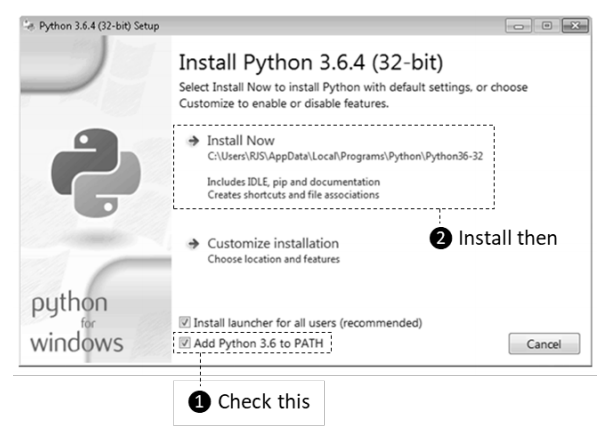
Download the latest Python 3 installer from Python.org (current version is 3.6.4). When starting the installer, use default settings, but make sure Python is added to your system's path variable (see Figure 1).
|
Step 2: Installing Jupyter
After Python has been installed, a command window needs to be opened. Press the Win + R keys on your keyboard, type cmd and press Enter. Afterwards, enter the following
line into the command window and press Enter again: pip install jupyter
Step 3: Installing R and the R kernel
Download the latest R installer from R-Project.org (current version is 3.4.4). Make sure to select the base installation for Windows. Run the installer using default settings afterwards.
Finally, Jupyter must be interconnected with R by installing the R kernel. Open the R console by starting R.exe (to be found under C:\Program Files\R\R-3.4.3\bin). Copy the following command into the console window and press enter: install.packages(c(’repr’, ’IRdisplay’, ’evaluate’, ’crayon’, ’pbdZMQ’, ’devtools’, ’uuid’, ’digest’))
This downloads a set of packages required by the R kernel. You may be asked to create a personal library; respond with "yes." If you are asked to select a CRAN mirror, select a mirror close to your current location, as this accelerates the download. While retrieving the packages, several warnings may be printed in the console window. They can be ignored. After all packages have been downloaded, execute the following command in the R console: devtools::install_github(’IRkernel/ IRkernel’)
This installs the R kernel. Upcoming warning messages can be ignored again. Afterwards, we need to make sure Jupyter identifies the newly installed kernel. Therefore, its spec must be registered by executing the following command in the R console: IRkernel::installspec()
Starting Jupyter
Now we are ready to start Jupyter. Close the R console and open a new Windows command prompt as explained in Step 2. Type jupyter notebook, then press Enter. Starting the notebook system may take some seconds. Afterwards, a browser window opens, showing Jupyter’s homepage (see Figure 2). Congratulations, Jupyter has been set up successfully. In case you want to shut down the notebook system, simply close the command window. Whenever you want to start it up again, open a new command window and repeat execution of the
jupyter notebook command.
|
Creating and editing a notebook
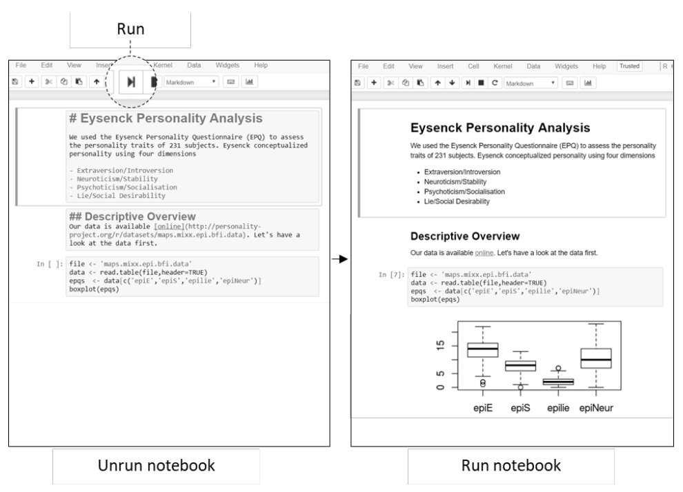
When looking at Jupyter’s home screen, you will see your computer’s user directory. By default, the notebook app can only access files within this directory and any subfolders. Navigate to a place where you want to store your notebooks. You can create a new folder by clicking New → Folder and renaming it afterwards by selecting it and clicking Rename. After choosing a folder, create a new notebook in there by clicking New → Notebook: R. A new browser window opens, showing the empty notebook you just created. Each notebook is made of vertically ordered cells holding either explanatory content or code. The input of each cell can be interpreted (i.e., run) by Jupyter, leading to a well-formatted output. Figure 3 shows an example. As we can see on the left side, this notebook contains multiple cells. When running them (by pressing the play button at the top of the page), they are rendered as shown on the right side.
|
In our empty notebook we can easily create new cells by clicking the plus button. Before filling the cells, we have to decide about the type of content. Each cell can be a Markdown or code cell. You can change the cell type by clicking Cell → Cell Type in the menu. To get a deeper understanding about the two types, we will use our recently created notebook for the analysis of exemplary Big Five personality data to be retrieved from the Personality Project. First, we will note down some conceptual basics using Markdown cells. Afterwards we will load the data and analyze it using code cells. As the algorithms may require some explanation, code cells should alternate with describing Markdown cells. The final result can be previewed and downloaded here. Before entering the first cell, let’s change the name of our empty notebook. Click on the title at the top of the page and change it to something like Working with Personality Data.
Markdown cells
Markdown cells are used for explanatory static content like text, images, and mathematical expressions. The content is styled and formatted by using the popular Markdown syntax. It is also possible to use HTML commands. Furthermore, mathematical expressions can be added to Markdown cells using LaTeX expressions. When Markdown cells are interpreted, their content is formatted by Jupyter and presented in an easy-to-read way. In summary, Markdown cells can be used to achieve a presentation of static content comparable to current psychological journal publications. Let’s have a closer look at some examples.
Heading, bold, and italic text
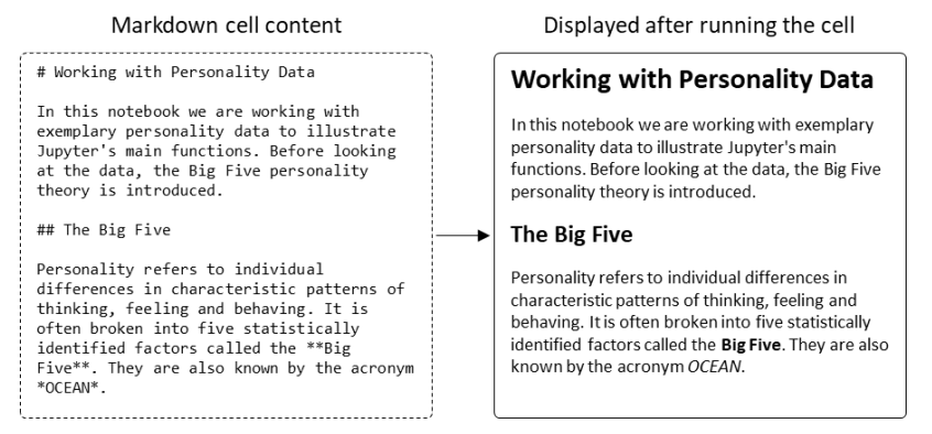
Headings can be used to structure texts. In Markdown, a heading has to be in its own line and preceded by hashtags (#). The amount of hashtags defines the outline level of a heading. Text can be decorated using bold or italic style. Letters, words, or groups of words surrounded by a single asterisk (*) are printed in italics, whereas using two asterisks (**) causes bold printing. Try to add the content shown on the left side of Figure 4 to your first Markdown cell. After running the cell, you should see a well-formatted output containing headings, as well as bold and italic text, as shown on the right side of the figure.
|
Links and images
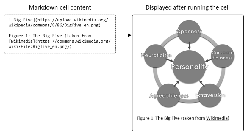
Links to websites or external data can be added to Markdown cells too. Simply surround the link’s name in square brackets, followed by the target address in round brackets. You can also include images to your notebook. To do that, use an exclamation mark (!), followed by an image title in square brackets and the image’s address in round brackets. If you want to show an image that is stored in the same location as your notebook, you do not need to provide its full address. Instead, you can just use its filename. Add another Markdown cell to your notebook containing the text from Figure 5. When running this cell, you should see both a link and an image of the Big Five retrieved from Wikimedia Commons.
|
Lists and tables
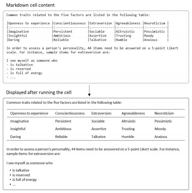
Markdown supports both numbered and unnumbered lists. Starting a new line of text with a number and a dot (1.) defines an item of a numbered list. Using a hyphen (-) instead defines an item of an unnumbered list. Tables can be rendered too, using a more complex syntax. Figure 6 shows an example. When you copy the text from the left side into a new Markdown cell, a table containing exemplary traits will be printed after running the cell. Furthermore, an unnumbered list of exemplary items will be rendered.
|
Mathematical expressions
Furthermore, Markdown can print mathematical expressions defined using LaTeX conventions. Simply surround the LaTeX-formatted expression with single dollar signs ($) to print it in line with encompassing text or double dollar signs ($$) to render it in a separate paragraph. Try to run the example presented in Figure 7.
|
Code cells
Code cells contain scripts written in a programming language like Python or (in our case) R. When interpreted by Jupyter, their output is presented below the respective cell. Depending on the languages and libraries used, outputs typically include tables, graphs (e.g., function plots, maps and rendered images), or even interactive elements like buttons and sliders. The latter can be used to alter variables within the code and visualize their effects on the output. In psychological research this can be used to investigate specific parameters of data preparation and analysis. Typical applications include the exploration of cutoff values and outlier limits, the visualization of different statistical methods and their effects, as well as the presentation of results. In comparison to Markdown cells, code cells are marked by the preceding keyword "In." Note that all code used within the same notebook has to be of the same language.
Let’s continue working on our personality data notebook. We already used Markdown cells to introduce the basic concept of the Big Five. Now we want to add code cells for loading real data and working with it. R provides several options for accessing both local and remote files. First, we can access data stored on our computer. For example, if a file data.csv containing personality data is stored in the exact same folder as our notebook, we can easily load its content into a new variable called person.data using the following two lines of code: filename <- ’data.csv’ person.data <- read.table(filename, header=TRUE)
Second, we can access any file being publicly available on the web. For example, we can use the following lines to retrieve data from Northwestern University’s Personality Project and store it in a new variable called person.data. Create a new code cell in your notebook containing these lines. Take care when copying the web address; it must not contain any spaces or line breaks. We enter:
filename <- ’http:// personality-project.org/r/datasets/ maps.mixx.epi.bfi.data’
person.data <- read.table(datafilename, header=TRUE)
To check if loading the data works as expected, also add the following line at the end of your code cell:
person.data
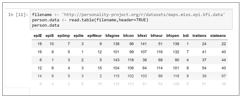
Run the cell (by clicking the Run button as shown in Figure 3, or by pressing Ctrl-Enter). The interpreter will load the data, create two new variables called "filename" and "person.data," and finally print parts of the content of person.data in a table below the code cell (see Figure 8).
|
As we can see, the loaded file contains different personality scales for a lot of subjects. Since we are interested in the Big Five, we should only use a subset of columns (those starting with "bf") for a subsequent analysis. Let’s create a new variable containing these columns by adding another code cell at the end of our notebook. Enter the following:
bigfive <- person.data[c(’bfagree’,’ bfcon’,’bfext’,’bfneur’,’bfopen’)]
boxplot(bigfive,las=2)
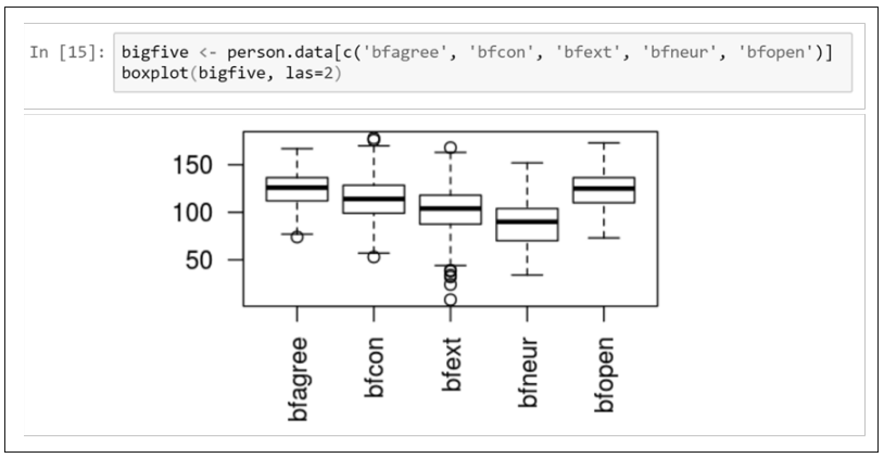
After running the cell, a boxplot will pop up below the code, showing descriptive details of the five factors (see Figure 9). Just like when working with plain R, data can be analyzed and manipulated in endless ways. You may have noticed that variables created after running a code cell are usable within the other code cells too. That’s why we could use the variable person.data to extract the Big Five.
|
Since Jupyter has no variable viewer, we need to use another code cell running the ls() command for getting an overview about the variables currently in use. By doing so, you will see that three variables have been created while we have been working with our notebook (filename, person.data and bigfive). If you want to delete all variables, you have to restart the R kernel from the menu by clicking Kernel → Restart. This is especially useful to clean up the notebook’s memory after experimenting with a lot of variables. Always remember to restart the kernel if you want to rerun the whole notebook from a defined starting point.
Advanced features
Jupyter provides useful tools we cannot cover in detail here. Cells can be split, merged, deleted, moved, and converted from one type to the other. They can be interpreted one by one or all at once. Notebooks can be exported into common formats including LaTeX, PDF, and HTML. Depending on the target format, this may require a working internet connection since conversion services from the web are used. All features are accessible over the extensive menu at the top of the notebook.
As of today, many plugins are available to extend the functionality of Jupyter. This includes additions for the management of references as well as plugins enabling others to comment on notebook content. Please consult the official Jupyter documentation about installing and using these plugins, available from http://jupyternotebook.readthedocs.io/.
Versioning and sharing notebooks
Jupyter makes it easy to keep track of our changes made to a notebook. It automatically saves an opened notebook from time to time, and we can force it to do so by clicking File → Save and Checkpoint. Jupyter allows us to restore a saved checkpoint by choosing File → Revert to Checkpoint. That means we can easily roll back to an older version after significant experimentation.
In many cases, you want to provide a notebook to other people. There are several options to share it. First, you can send the notebook file via email. The receiving person can simply load the notebook in his or her own Jupyter installation by choosing File → Open from the menu. Second, you can host your notebook online and provide its link to others, so they can continue where you finished working. You can either bring your own Jupyter installation online (this requires setting up a server machine and cannot be detailed here) or use an installation set up by one of several specialized cloud hosting providers (e.g., Microsoft Azure Notebooks). However, it is not possible to bring your notebooks online by using file hosting platforms like Dropbox or Google Drive. Since Jupyter is still in its infancy, alternatives for sharing notebooks are expected to increase.
Conclusion
Jupyter is designed to solve some of the main problems in psychological research. First, it helps scientists keep track of their work. Since both static and dynamic assets of a research project can be included in Jupyter notebooks, they help organize ideas, information acquired from lab or field environments, statistical methods and scripts, as well as results and interpretations. Everything is kept in one place. Changes are documented and can be reverted at any time. Second, Jupyter promotes sharing work. It enables others to explore and understand the research undertaken. Thus, Jupyter may help increase the reproducibility of results and foster good academic practice.
However, there are other notebook systems as well. This includes Apache Zepplin and the R Notebooks feature of RStudio. Apache Zeppelin is a web-based notebook system like Jupyter. It was designed for data analysis using Python and Spark, but can be used with R too. Apache Zeppelin even supports combining several languages within the same notebook, a feature missing in Jupyter. Unfortunately, setting up Apache Zeppelin on a Windows machine requires a lot of effort. The system is pretty new and not as well established as Jupyter. Thus, Jupyter may be the better choice. However, if you are familiar with RStudio and use R for all your data analysis, you won’t need Jupyter at all. RStudio supports writing R Notebooks containing both markup and R code. The notebooks can be shared more easily, compared to Jupyter, because they are stored as plain text. Unfortunately, R Notebooks do not support coding in other languages. In conclusion, for Windows users with the need for multiple languages, Jupyter notebooks may be the best choice. In any case, they are a great addition to the often short and abstract journal publications.
References
- ↑ Klein, R.A.; Ratliff, K.A.; Vianello, M. et al. (2014). "Investigating Variation in Replicability: A “Many Labs” Replication Project". Social Psychology 45 (3): 142–52. doi:10.1027/1864-9335/a000178.
- ↑ Pashler, H.; Wagenmakers, E.J. (2012). "Editors' Introduction to the Special Section on Replicability in Psychological Science: A Crisis of Confidence?". Perspectives on Psychological Science 7 (6): 528-30. doi:10.1177/1745691612465253. PMID 26168108.
- ↑ Yong, E. (2012). "Replication studies: Bad copy". Nature 485 (7398): 298-300. doi:10.1038/485298a. PMID 22596136.
- ↑ Nosek, B.A.; Spies, J.R.; Motyl, M. (2012). "Scientific Utopia: II. Restructuring Incentives and Practices to Promote Truth Over Publishability". Perspectives on Psychological Science 7 (6): 615-31. doi:10.1177/1745691612459058. PMID 26168121.
- ↑ Donoho, D.L.; Maleki, A.; Rahman, I.U. et al. (2009). "Reproducible Research in Computational Harmonic Analysis". Computing in Science & Engineering 11 (1): 8-18. doi:10.1109/MCSE.2009.15.
- ↑ Shen, H. (2014). "Interactive notebooks: Sharing the code". Nature 515 (7525): 151–2. doi:10.1038/515151a. PMID 25373681.
- ↑ Perez, F.; Granger, B.E. (2007). "IPython: A System for Interactive Scientific Computing". Computing in Science & Engineering 9 (3): 21–9. doi:10.1109/MCSE.2007.53.
Notes
This presentation is faithful to the original, with only a few minor changes to presentation. In some cases important information was missing from the references, and that information was added. The original article lists reference alphabetically; this version lists them in order of appearance, by design.
